TheCodeBuzz

Today in this article, we will see the Cassandra best practices that matter for a production cluster. We cover data modeling, consistency and day-2 operations, so you can design the cluster and also keep it healthy after go-live.

The scope includes query-first modeling, partition key design, Storage-Attached Indexes (SAI), consistency levels, lightweight transactions (LWT) and Accord, tombstones, compaction, drivers, security, repair, backups, monitoring and upgrades. Every rule comes with the reason behind it, so you can judge when it fits your workload and when it does not.

Many popular guides still carry pre-5.0 advice. This guide adds what they often miss: the limits of SAI, UCS versus the STCS default, repair tied to gc_grace_seconds, driver settings, security and restore testing. It is written for engineers, architects and DBAs who run Cassandra in production.

For the version baseline, Apache Cassandra 5.0 is the latest GA series (5.0.9, released 2026-08-07), and 4.1 is the previous stable line (4.1.12). The 3.x series is end-of-life. Cassandra 6.0 is still pre-GA (6.0-alpha3) and is not for production.

Version note: This guide targets Apache Cassandra 5.0.9 (latest GA) and 4.1.12 (previous stable line), and treats 6.0-alpha3 as pre-GA only.

 

In this guide

 

• Cassandra Best Practices at a Glance
• Cassandra Data Modeling Best Practices and Partition Key Design
• Indexing in Cassandra 5.0: SAI, Secondary Indexes or More Tables
• Consistency Levels and Replication Factor: Choosing LOCAL_QUORUM
• Transactions and Lightweight Transactions: Paxos v2 and Accord in Cassandra 6.0
• Tombstones, TTL and gc_grace_seconds: Deleting Data Safely
• Choosing a Compaction Strategy: STCS, LCS, TWCS or UCS
• Drivers, Connection Management and Security
• Repair, Backup and Restore Best Practices
• Operations, Monitoring and Upgrades
• Common Cassandra Anti-Patterns
• Cassandra Production Readiness Checklist
• Key takeaways
• FAQ

Cassandra Best Practices at a Glance

Apache Cassandra is a distributed, wide-column database built for high write throughput and availability across nodes and datacenters. Today in this guide, we will see Cassandra data modeling best practices, consistency, indexing, repair, backups and upgrades in one place.

Note: A partition is like one drawer in a filing cabinet. Every row with the same partition key goes into the same drawer, and that drawer lives on specific nodes. Unlike a real cabinet, each drawer is copied to several nodes, so one failure doesn’t lose it.

Best Practices Summary Table

The table below lists the main areas, what to do and what to avoid. Each row is explained in its own section later.

Area	Do this	Avoid this
Data modeling	Model one table per query and denormalize.	Designing tables from entities and expecting joins.
Partition key	Use a high-cardinality key and keep partitions under about 100 MB and 100,000 items.	Low-cardinality keys (e.g. country, status) and unbounded partitions.
Indexing	Use extra tables for hot queries and SAI for secondary lookups.	Legacy secondary indexes in new designs.
Consistency	Use LOCAL_QUORUM for reads and writes in multi-datacenter clusters.	ALL, or cross-datacenter QUORUM by default.
Replication factor	Use RF=3 per datacenter with NetworkTopologyStrategy.	SimpleStrategy in multi-datacenter production.
Transactions	Use LWT only for compare-and-set on one partition.	LWT as the default write path.
Deletes and TTL	Prefer TTL and time bucketing over explicit deletes.	Queue-style tables and explicit null writes.
Compaction	Pick a strategy per table (UCS, or TWCS for TTL-heavy time series).	Leaving every table on the default without review.
Drivers	Use one long-lived session, prepared statements and an explicit local datacenter.	One session per request.
Security	Enable authentication, authorization and TLS, and replace the default superuser.	Running with defaults open.
Repair	Finish repair inside gc_grace_seconds (default 864000 seconds, 10 days).	Rare or skipped repair.
Backups	Schedule snapshots, store them off the node and test restores.	Snapshots that were never restored.
Monitoring	Watch partition size, pending compactions, latency and dropped messages.	Looking only at CPU and disk.
Upgrades	Move off 3.x because it is end-of-life, and roll one node at a time.	Staying on 3.x or running pre-GA builds.

Which Cassandra Version Does This Guide Assume?

This guide uses the versions below as its baseline.

• 5.0.9: the latest GA release, and the preferred target.
• 4.1.12: the latest on the previous stable line.
• 6.0-alpha3: pre-GA and not for production.
• Java: Java 11 and 17 are used with Cassandra 5.0.x.

Cassandra Data Modeling Best Practices and Partition Key Design

Design your tables from your queries, not from your entities. A good Cassandra model has three goals: spread data evenly with a high-cardinality partition key, bound partition size, and read as few partitions as possible, ideally one per query.

Why should a query read only one partition?

A single-partition read goes to the replicas that own that partition. A multi-partition read makes the coordinator (the node handling the request) contact several nodes and wait for the slowest one. That adds latency variance, so the occasional slow response hurts your tail latency.

How do you choose the partition key and clustering columns?

The partition key decides which nodes hold the data. Clustering columns decide the sort order of rows inside that partition. Pick the partition key from the column your query always filters by with equality, and pick clustering columns from the sort or range you need.

Example: a retail app shows “my orders, newest first”. The table below shows how the choice maps.

Part	Column	Why
Partition key	customer_id	High cardinality, and every query supplies it
Clustering column	order_date DESC	Newest orders are read first, with no sorting at query time
Clustering column	order_id	Keeps rows unique when two orders share a timestamp

How big should a partition be?

Keep partitions under about 100 MB and under about 100,000 items. The hard practical limit is 2 billion cells per partition, but you should never plan to get near it.

Oversized partitions hurt in several ways:

• Heavy reads: the node must scan and merge more data for each request.
• Compaction and repair pressure: large partitions take longer to merge and to compare between replicas.
• Hot nodes: one partition lives on only a few replicas, so one big partition loads those nodes unevenly.

How does bucketing keep partitions bounded?

Bucketing means adding a column, such as a day or hour, to the partition key so a busy key stops growing forever. One IoT sensor writing every second would otherwise build a single unbounded partition.

In plain English: Think of a ledger where you start a new page every day. You never end up with one endless page, and you can still find any day quickly. The catch is that a question spanning ten days means opening ten pages.

Here is a simplified sensor table with a day bucket in the partition key, followed by a single-partition read:

CQL

CREATE TABLE iot.sensor_readings (
    sensor_id    text,
    day_bucket   date,
    reading_time timestamp,
    temperature  double,
    PRIMARY KEY ((sensor_id, day_bucket), reading_time)
) WITH CLUSTERING ORDER BY (reading_time DESC);

SELECT reading_time, temperature
FROM iot.sensor_readings
WHERE sensor_id = 'sensor-1001'
  AND day_bucket = '2026-10-20'
LIMIT 100;

✅ One partition, newest readings first, and each partition holds at most one day of data per sensor.

The trade-off: a query over several days now touches several partitions. The application must list the buckets and query each one explicitly (e.g. seven queries for a week). Choose a bucket size so a partition stays within the limits above at your peak write rate.

What are hot partitions and how do you avoid them?

A hot partition is one that receives a disproportionate share of traffic. Low-cardinality keys such as country or status create them, because millions of rows share a few key values and land on a few nodes. Use a key with many distinct values, and add a bucket if one value is still very busy.

Is denormalization normal in Cassandra?

Yes. Cassandra has no joins, so you store the same data in several tables, one per query (e.g. orders_by_customer and orders_by_date). One write to several tables is cheaper than a read that must gather data from many partitions.

Use a logged batch only to keep those denormalized tables in sync, because it guarantees all writes eventually apply. Don’t use it for speed. A batch across many partitions adds work on the coordinator.

Why avoid ALLOW FILTERING and full scans?

ALLOW FILTERING lets a query run without a full partition key, so Cassandra reads many partitions and discards rows that don’t match. Cost grows with table size, and latency becomes unpredictable. Keep it out of application paths. If you need the query often, create a table for it instead.

Indexing in Cassandra 5.0: SAI, Secondary Indexes or More Tables

Use denormalized tables for hot, latency-critical queries. Use Storage-Attached Indexes (SAI), new in Cassandra 5.0, for secondary lookups where a partition-key query is not possible. Avoid legacy secondary indexes (2i) in new designs.

What is SAI in Cassandra 5.0?

SAI is an index attached to the SSTables of a table. It lets you filter on non-key columns without creating a separate table. The 5.0 feature list also includes a vector data type with similarity functions, which builds on SAI.

In plain English: A denormalized table is a second filing cabinet sorted the way you search. SAI is a small index card stapled to each existing drawer, so you can look things up by another field. The cards help, but you still have to know which drawers to open.

Denormalized table, SAI or legacy index?

The table below compares the three options across cost and limits.

Option	Read cost	Write cost	Storage	Best fit	Limits
Denormalized table	Lowest, single partition	One extra write per table	Full copy of the data	Primary, latency-critical queries	App must keep copies in sync
SAI	Low with a partition restriction, variable without	Index update on write	Index files per SSTable	Secondary filters on non-key columns	Does not replace query-first modeling
Legacy 2i	Often high, can hit many nodes	Index update on write	Hidden local index table	Rarely a good choice	Poor with high-cardinality columns

What are the limits of SAI?

An SAI query with no partition key may fan out across nodes, so it adds latency variance. SAI does not remove the need for Cassandra data modeling best practices. Test every SAI query on production-size data before you rely on it, because small test sets hide fan-out cost.

When should you pick which?

• Primary query: “orders by customer” is the main read path, so build it as a table keyed by customer.
• Secondary filter: “find orders by status in this customer’s partition” is fine with SAI plus a partition restriction (e.g. a retail support screen).
• Cross-partition search: Use SAI only if the latency variance is acceptable. Otherwise add another table.

Here is a simplified example that indexes the status column and queries it inside one customer partition:

CQL

CREATE TABLE IF NOT EXISTS shop.orders_by_customer (
  customer_id uuid,
  order_id timeuuid,
  status text,
  total decimal,
  PRIMARY KEY ((customer_id), order_id)
) WITH CLUSTERING ORDER BY (order_id DESC);

CREATE INDEX IF NOT EXISTS orders_status_sai
  ON shop.orders_by_customer (status) USING 'sai';

SELECT order_id, status, total
FROM shop.orders_by_customer
WHERE customer_id = 7b1f3c52-8a6e-4c1d-9d0e-3f2a5b6c7d88
  AND status = 'SHIPPED';

The query returns only the shipped orders for that one customer. The partition key restriction keeps it on the replicas of a single partition, and SAI handles the status filter.

Consistency Levels and Replication Factor: Choosing LOCAL_QUORUM

For most multi-datacenter production workloads, use RF=3 per datacenter with LOCAL_QUORUM for both reads and writes. RF=3 lets a quorum form from two agreeing replicas, tolerates one node failure and allows rolling restarts without downtime.

What is a consistency level?

A consistency level is the number of replicas that must confirm a read or write before Cassandra reports success to the client. You choose it per request, so different queries can make different trade-offs.

Note : Three people hold a copy of the same record. A consistency level decides how many of them must say “done” before you accept the answer, like a committee that needs a majority vote. The analogy stops fitting in one place: Cassandra still sends the write to all copy-holders, it only waits for some of them.

How do QUORUM and LOCAL_QUORUM differ?

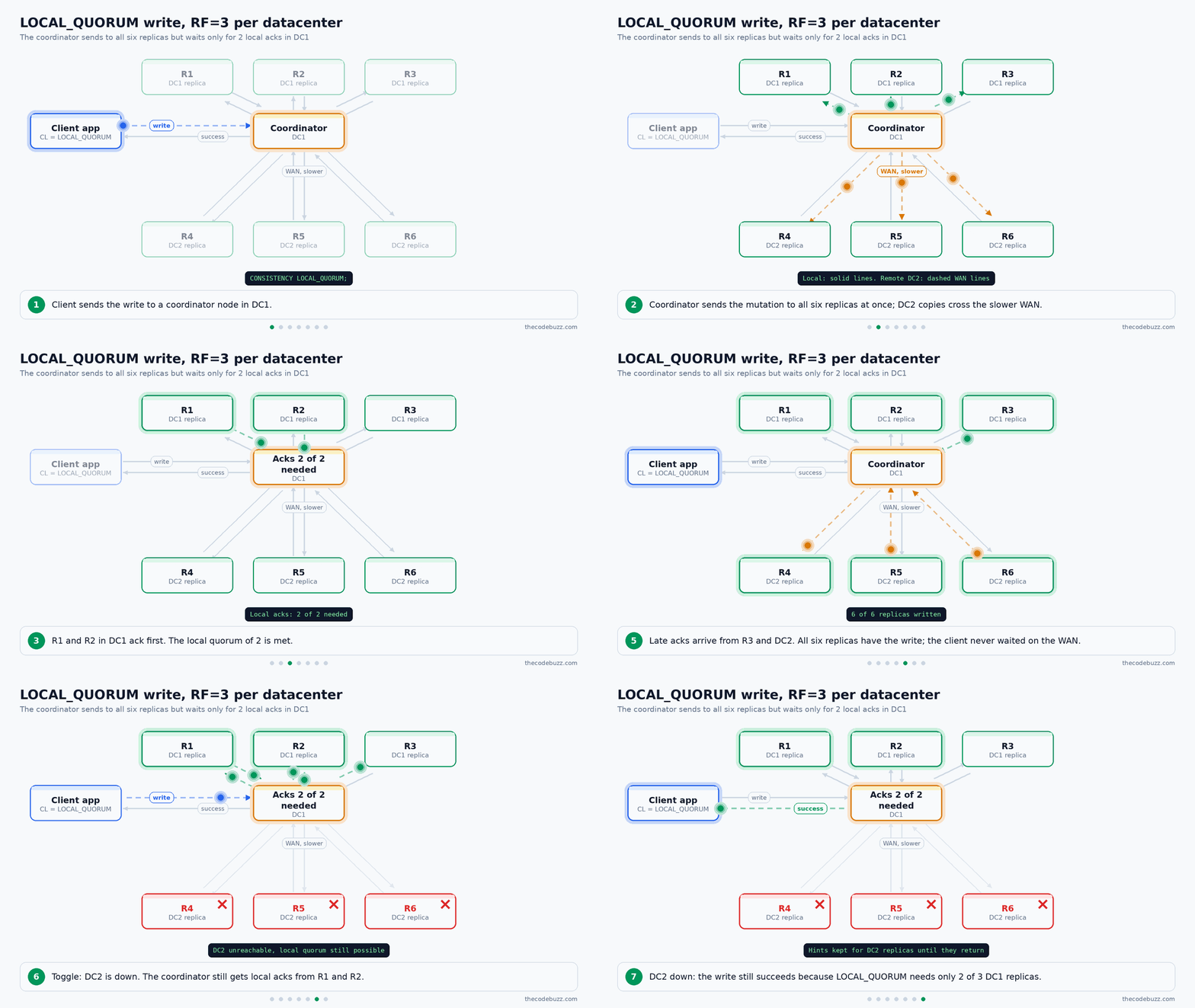
QUORUM needs RF/2 + 1 replicas (integer division) across all datacenters. LOCAL_QUORUM needs a majority only in the coordinator’s datacenter, which is 2 of 3 with RF=3.

With two datacenters at RF=3, there are six replicas in total, so QUORUM needs four. That forces at least one cross-datacenter acknowledgment. LOCAL_QUORUM avoids that WAN latency and keeps working if the other datacenter is completely down. The animated diagram below shows a LOCAL_QUORUM write, including the case where DC2 is unavailable.

Which consistency level fits which use case?

The table assumes two datacenters with RF=3 each (six replicas in total).

Level	Replicas needed	Latency	Availability	Typical use
ONE	1, any DC	Lowest	Highest	Data where stale reads are fine
LOCAL_ONE	1, local DC	Lowest, no WAN	High	Low-value reads in one DC
QUORUM	4 of 6	Includes WAN	Medium	Single-DC clusters, cross-DC strictness
LOCAL_QUORUM	2 of 3 local	Low, no WAN	High	Default for multi-DC production
EACH_QUORUM (writes only)	2 of 3 in each DC	High	Low	Rare writes that must reach every DC
ALL	6 of 6	Highest	Lowest	Almost never

When do you get strong consistency?

You get strong consistency when read replicas plus write replicas is greater than RF. With RF=3, LOCAL_QUORUM on both sides gives 2 + 2 = 4, which is more than 3, so every read overlaps at least one replica that saw the latest write. This gives read-your-writes within that datacenter.

Know the trade-offs. ALL fails as soon as one replica is down, so one node restart becomes an outage. ONE is fast but can return stale data. Use lower levels only where staleness is acceptable, such as video view counters on a media site. Use LOCAL_QUORUM for order and payment data in a retail system.

How do you set replication correctly?

Use NetworkTopologyStrategy with an explicit RF per datacenter, and make sure the snitch reports correct datacenter and rack names. Do not use SimpleStrategy in production multi-datacenter clusters, because it ignores topology and can place all replicas in one rack or datacenter.

The example below creates a keyspace with RF=3 in each datacenter, then sets the session consistency in cqlsh:

CQL

CREATE KEYSPACE retail
  WITH replication = {
    'class': 'NetworkTopologyStrategy',
    'dc1': 3,
    'dc2': 3
  };

CONSISTENCY LOCAL_QUORUM;

Each datacenter keeps three replicas, and every later read or write in this cqlsh session waits for two local replicas. The names dc1 and dc2 must match the datacenter names your snitch reports.

Transactions and Lightweight Transactions: Paxos v2 and Accord in Cassandra 6.0

Cassandra gives you atomicity and isolation per partition. For compare-and-set on a single partition it offers lightweight transactions (LWT, written as IF conditions). It is not a general ACID database today.

When should you use a lightweight transaction?

Use LWT only where two writers must not both succeed, such as a unique username or an inventory reservation. Paxos, the consensus protocol behind LWT, needs several round trips between replicas, so it costs far more than a normal write. Don’t make it your default write path.

In plain English: A normal write is like dropping a note in a mailbox. An LWT is like getting every committee member to agree out loud before the note is filed. It is safer, but it takes much longer.

Example: a bank checks that an email is unused before opening an account. The check and the insert must happen as one step, as shown below.

CQL

CREATE TABLE IF NOT EXISTS bank.users_by_email (
  email text PRIMARY KEY,
  user_id uuid,
  created_at timestamp
);

SERIAL CONSISTENCY LOCAL_SERIAL;

INSERT INTO bank.users_by_email (email, user_id, created_at)
VALUES ('asha@example.com', uuid(), toTimestamp(now()))
IF NOT EXISTS;

The result has an [applied] column. True means the row was inserted. False means the email already exists, and the existing row is returned. Always check this column in your application code. LOCAL_SERIAL limits the Paxos phase to the local datacenter, and SERIAL spans all datacenters.

Which Paxos settings should you set in production?

Set paxos_variant to v2 together with paxos_state_purging set to repaired. The two settings are independent, so set both deliberately. Test the change in staging and follow the official upgrade notes for your exact version.

What does Accord in Cassandra 6.0 add?

Accord adds multi-partition, strict-serializable transactions through BEGIN TRANSACTION. Cassandra 6.0 is still pre-GA (6.0-alpha3), and Accord is beta and off by default. It requires Transactional Cluster Metadata and doesn’t support counter tables. It also rejects LOCAL_QUORUM, TWO and THREE for Accord operations. Don’t plan production designs on it yet, because 5.0.9 remains the current GA release.

Plain writes, logged batch, LWT or Accord: how do they compare?

This table compares the four options by scope, isolation, cost and status.

Option	Scope	Isolation	Cost	Status
Plain write	Single partition	Per partition	Lowest	GA
Logged batch	Multiple tables or partitions	Eventual all-or-nothing, no cross-partition isolation	Extra batchlog writes	GA
LWT	Single partition, conditional	Serializable per partition	Several round trips	GA
Accord	Multiple partitions	Strict serializable	Not benchmarked here	Beta, 6.0 pre-GA

Tombstones, TTL and gc_grace_seconds: Deleting Data Safely

A delete in Cassandra writes a tombstone, a marker saying the data is deleted, instead of removing it right away. Tombstones are purged only after gc_grace_seconds (default 864000 seconds, 10 days) has passed and only when compaction runs. Until then, reads must scan them, so heavy deletes slow reads.

In plain English: A tombstone is a crossed-out line in a ledger. The old line stays on the page, and the crossing-out is only cleaned up when the ledger is rewritten. Unlike a ledger, Cassandra keeps copies on several nodes, and every copy must see the crossing-out.

Why must repair finish within gc_grace_seconds?

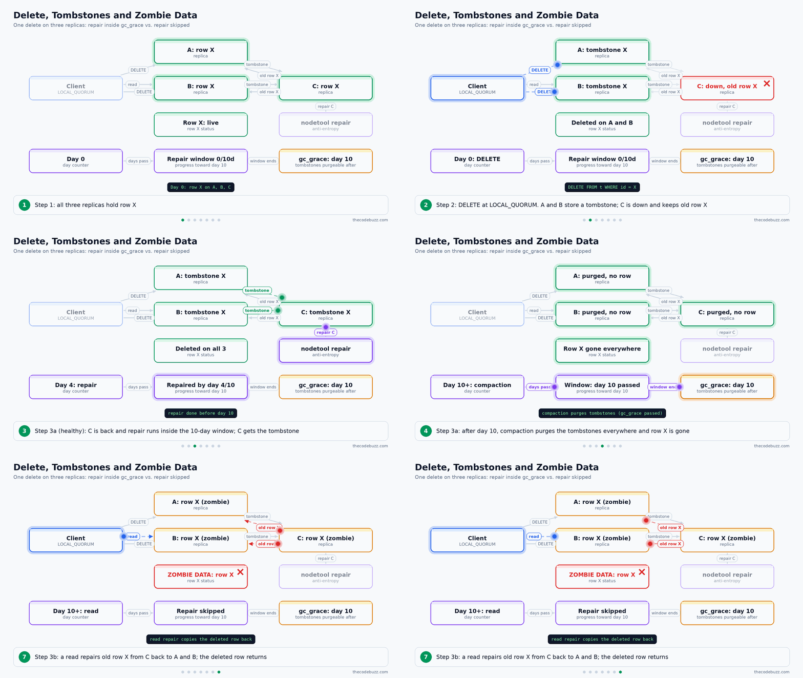
If a replica misses a delete and the other replicas purge their tombstones, that replica becomes the only holder of the row. The next read or repair copies the old value back, and the deleted row returns as zombie data. Repair inside the grace window prevents this.

The animated diagram below shows a delete across three replicas, with the healthy path and the zombie failure path side by side.

What creates tombstones?

These patterns produce most tombstone problems in production:

• Queue-style tables: rows are inserted, read and deleted in the same partition, so reads scan many dead entries.
• Frequent deletes: every delete adds a marker that stays for at least the grace period.
• Partial deletes in wide partitions: row or range deletes inside a large partition leave many markers next to live data.
• Null writes: explicitly inserting null writes a tombstone. Leave the column out of the statement, or pass the driver’s unset value (e.g. UNSET_VALUE in the Python driver).

How do you delete data safely?

1. Use TTL instead of DELETE: let data expire on its own schedule. Cassandra 5.0 also extends the maximum TTL, which helps for long retention.
2. Bucket by time: put a day or hour bucket in the partition key so old data sits in partitions you stop reading.
3. Avoid large range deletes: they leave wide tombstones that every read must check.
4. Use TWCS for TTL-heavy data: when data is time-windowed and not updated out of order, whole expired SSTables can be dropped.

Example: a retail site keeps cart-activity events for seven days. TTL plus TWCS removes them without any application delete.

CQL

CREATE TABLE shop.cart_events (
    user_id    uuid,
    day_bucket date,
    event_time timestamp,
    event_type text,
    PRIMARY KEY ((user_id, day_bucket), event_time)
) WITH CLUSTERING ORDER BY (event_time DESC)
  AND default_time_to_live = 604800
  AND compaction = {
    'class': 'TimeWindowCompactionStrategy',
    'compaction_window_unit': 'DAYS',
    'compaction_window_size': 1
  };

INSERT INTO shop.cart_events (user_id, day_bucket, event_time, event_type)
VALUES (uuid(), '2026-10-20', toTimestamp(now()), 'add_to_cart')
USING TTL 86400;

The table default expires rows after seven days, and the insert overrides it with a one-day TTL. Each daily window becomes its own SSTable group that can be dropped as a whole.

How do you catch tombstone problems early?

Set the tombstone warn and failure thresholds in cassandra.yaml and review the guardrails available in your version. Check nodetool tablestats for average and maximum tombstones per slice, and watch the logs for tombstone warnings.

Warning: Don’t lower gc_grace_seconds just to purge faster. A shorter value frees space sooner, but it raises the risk of zombie data unless repair completes more often than the new value. Lower it only after your repair schedule is proven to beat it.

Choosing a Compaction Strategy: STCS, LCS, TWCS or UCS

STCS is still the default in Cassandra 5.0, but the UCS documentation recommends the Unified Compaction Strategy (UCS) for most workloads. UCS can also be configured to behave like the older strategies. If you stay on classic strategies, use TWCS for TTL-heavy time-series data.

What does compaction do?

Compaction is the background process that merges SSTables (the immutable data files on disk) to drop overwritten data and expired tombstones. The strategy you pick decides which files get merged and when.

In plain English: Think of many small notebooks piling up on a desk. Compaction copies the latest notes into fewer, cleaner notebooks and throws the old ones away. The strategy is the rule for which notebooks you tidy together, and how often.

How do the four strategies compare?

The animated diagram below walks through the decision for one table, and the table after it compares the strategies in qualitative terms.

Strategy	Best for	Read amplification	Write amplification	Space overhead	Watch out for
STCS	Write-heavy, general use	Higher	Lower	Higher	Large compactions need spare disk
LCS	Read-heavy, strict latency	Lower	Higher	Lower	Heavy write I/O
TWCS	TTL time-series	Low for recent windows	Lower	Low when expiry works	Out-of-order updates and deletes
UCS	Most workloads	Tunable	Tunable	Tunable	Check parameters for your version

Why do the strategies behave differently?

• LCS: keeps data in small sorted levels, so a read touches few files. You pay with more write I/O.
• STCS: favors writes by merging files of similar size. Large merges need free disk space while they run.
• TWCS: groups data into time windows and drops a whole SSTable once everything in it has expired. This only works if data isn’t updated or deleted out of order.

How do you migrate a table to UCS?

1. Test first: try the change on a non-production cluster with realistic data.
2. Change per table: use ALTER TABLE, one table at a time.
3. Mimic your current strategy: start with settings that behave like STCS or LCS, then tune.
4. Watch the switch: track pending compactions and disk use while it runs.

Parameter names and defaults can change between versions, so confirm them in the official UCS documentation for your release. The T4 value below is the STCS-like setting from the 5.0 docs.

CQL

-- UCS, configured to behave like STCS
ALTER TABLE shop.orders_by_customer
WITH compaction = {
  'class': 'UnifiedCompactionStrategy',
  'scaling_parameters': 'T4'
};

-- TWCS for TTL-heavy time-series data
ALTER TABLE iot.sensor_readings
WITH compaction = {
  'class': 'TimeWindowCompactionStrategy',
  'compaction_window_unit': 'DAYS',
  'compaction_window_size': 1
};

Each statement changes the strategy for one table only. Then check progress on each node:

bash

nodetool compactionstats

This shows pending tasks and running compactions. A pending count that keeps growing after the switch means the node can’t keep up.

Cassandra 5.0 also adds trie memtables and trie SSTables. They are separate storage features from compaction, and you can evaluate them on their own.

Drivers, Connection Management and Security

Use one long-lived session per application, prepared statements, token-aware and datacenter-aware load balancing, and an explicitly set local datacenter. Turn on authentication, authorization and TLS from day one, because adding them later means a risky rolling change on a live cluster.

How should you manage connections?

Create the Session once at startup and share it across all requests. Opening one per request wastes connections and adds handshake latency. A prepared statement is parsed once on the server, and it lets the driver work out which replicas own the partition.

In plain English: Token-aware routing is like a courier who knows which house holds the parcel and goes straight there, instead of leaving it at a front desk that must pass it on. The “front desk” is the coordinator, and skipping it saves one network hop.

Set the local datacenter explicitly so traffic never reaches a remote DC by accident. Enable retries and speculative execution (sending a second request when the first is slow) only for idempotent statements, meaning ones that are safe to run twice.

The table below lists the driver settings to check, with the value to use and the reason:

Setting	Recommended	Reason
Local datacenter	Set explicitly (e.g. dc1)	Keeps requests out of remote DCs
Load balancing	Token-aware over DC-aware	Sends requests to a replica directly
Prepared statements	Always, for repeated queries	Parsed once, enables token routing
Retry and idempotence	Mark idempotent statements only	Avoids duplicate non-idempotent writes
Default consistency level	LOCAL_QUORUM	Matches RF=3 per DC, no cross-DC wait
Timeouts	Set client timeout above server timeout	Stops hung requests piling up

How do you configure the Python driver?

Here is a simplified example using ExecutionProfile, the current way to set policies and consistency:

Python

import os
import ssl
from cassandra import ConsistencyLevel
from cassandra.auth import PlainTextAuthProvider
from cassandra.cluster import Cluster, ExecutionProfile, EXEC_PROFILE_DEFAULT
from cassandra.policies import DCAwareRoundRobinPolicy, TokenAwarePolicy

profile = ExecutionProfile(
    load_balancing_policy=TokenAwarePolicy(DCAwareRoundRobinPolicy(local_dc="dc1")),
    consistency_level=ConsistencyLevel.LOCAL_QUORUM,
    request_timeout=5.0,
)

cluster = Cluster(
    ["10.0.0.1", "10.0.0.2"],
    auth_provider=PlainTextAuthProvider("app_user", os.environ["CASS_PASSWORD"]),
    ssl_context=ssl.create_default_context(cafile="ca.pem"),
    execution_profiles={EXEC_PROFILE_DEFAULT: profile},
)
session = cluster.connect("shop")  # create once, reuse everywhere

stmt = session.prepare("SELECT * FROM orders_by_customer WHERE customer_id = ?")
stmt.is_idempotent = True
rows = session.execute(stmt, [customer_id])

✅ One shared session, local DC set, LOCAL_QUORUM by default, TLS on, and a prepared read marked idempotent.

How do you configure the C# driver?

With the DataStax C# driver (CassandraCSharpDriver), build the Cluster once and register the session as a singleton:

C#

using Cassandra;

var cluster = Cluster.Builder()
    .AddContactPoints("10.0.0.1", "10.0.0.2")
    .WithLocalDatacenter("dc1")
    .WithCredentials("app_user", Environment.GetEnvironmentVariable("CASS_PASSWORD"))
    .WithSSL()
    .Build();

var session = await cluster.ConnectAsync("shop"); // singleton

var prepared = await session.PrepareAsync(
    "SELECT * FROM orders_by_customer WHERE customer_id = ?");

var bound = prepared.Bind(customerId)
    .SetConsistencyLevel(ConsistencyLevel.LocalQuorum)
    .SetIdempotence(true);

RowSet rows = await session.ExecuteAsync(bound);

The local DC is named, the statement is prepared and bound, and consistency is LocalQuorum.

How do you secure a Cassandra cluster?

Enable PasswordAuthenticator and CassandraAuthorizer in cassandra.yaml. Create your own superuser, then disable or drop the default cassandra role. Give each application a role with only the permissions it needs.

CQL

CREATE ROLE analyst WITH PASSWORD = 'use-a-strong-secret' AND LOGIN = true;
GRANT SELECT ON KEYSPACE clinic TO analyst;

• TLS: Enable client-to-node and node-to-node encryption. Use mutual TLS where you control the clients.
• Dynamic data masking (5.0): Hides sensitive column values from roles without unmask rights. Example: mask patient identifiers for analyst roles in a healthcare system.
• CIDR authorizer (5.0): Limits which networks a role can connect from.
• Guardrails: Added in 4.1 and extended in 5.0, they set warn and fail limits that stop risky operations, such as oversized partitions or too many tables.

Repair, Backup and Restore Best Practices

Run repair on every node within each gc_grace_seconds window. With the default of 864000 seconds that means at least once every 10 days, and in practice more often to leave a safety margin. Take scheduled snapshots with retention, enable commit log archiving for point-in-time restore, and test restores regularly.

What does Cassandra repair do?

Repair compares the replicas of the same data using Merkle trees (hash trees that summarize ranges of data) and streams any differences between nodes. It fixes data that a replica missed, for example while the node was down.

In plain English: Three people each keep a copy of the same notebook. Repair is the meeting where they compare page summaries, find pages that differ, and fill in the gaps. Unlike real people, the nodes compare hashes first, so they only copy the pages that really differ.

How should you schedule repair?

Run repair regularly in small pieces instead of rarely in one large job. Follow these rules:

• Prefer incremental repair: on versions that support it, it only checks data not yet repaired. Use full repair only when the release notes or a recovery task call for it.
• Use -pr on every node: the primary-range option repairs only the ranges a node owns first, so the same data isn’t compared three times.
• Go node by node: running repair on all nodes at once adds heavy streaming and compaction load.
• Automate it: open-source Cassandra has no NodeSync equivalent from DSE. Auto Repair (built-in scheduling) arrived in the 5.0.8+ backport and needs explicit opt-in. Otherwise use an external scheduler. Verify against the release notes for your exact version before enabling.
• Watch TTL-heavy tables: expired data becomes tombstones, and a replica that missed one can bring old values back after the purge. This is the same zombie-data risk described in the tombstones section.

Here is a simplified example of repairing the primary ranges of one keyspace on the current node:

BASH

nodetool repair -pr shop_ks

✅ Repairs only the ranges this node owns. Repeat on the next node when it finishes.

Which backup method should you use?

Use snapshots as the base and add commit log archiving if you need point-in-time recovery. The table compares the four common methods:

Method	What it gives you	Restore path	Limit
nodetool snapshot	Consistent point-in-time copy of SSTables per node	Copy files back or stream them	Only as fresh as the last run; lives on the same disk until you copy it away
Incremental backups	Hard links to SSTables flushed since the last snapshot	Restore the snapshot, then add the new files	Files pile up until you move and clean them
Commit log archiving	Writes between snapshots, for point-in-time restore	Replay logs up to a chosen timestamp	Needs archive and restore commands configured in advance
sstableloader / nodetool refresh	Loading tools, not backups	Stream (sstableloader) or copy files (refresh)	Needs the schema to exist first

Take a named snapshot, then copy it off the node:

BASH

nodetool snapshot -t daily_2026-10-20 shop_ks

Creates a snapshot tagged daily_2026-10-20 for every table in shop_ks. Store it off the node, because a snapshot on the same disk does not survive disk loss.

How do you restore and test a backup?

Restore the schema first, then the data, then run repair. The animated diagram below shows the full restore flow, step by step.

A restore test loads schema, snapshot SSTables and archived commit logs into a fresh cluster, then repairs and validates row counts against the source.

1. Restore the schema: apply the saved CQL so tables exist.
2. Load the data: stream SSTables with sstableloader, or copy files into the table directory and run nodetool refresh.
3. Replay commit logs: stop at the target timestamp for point-in-time recovery.
4. Repair and validate: run repair, then compare row counts with the source.

BASH

sstableloader -d 10.0.1.11,10.0.1.12 /restore/shop_ks/orders_by_customer

Streams the SSTables in that directory to the live cluster. The path must end in keyspace/table.

A backup that was never restored is untested. Run the restore on a separate cluster on a schedule, and time it. For example, a retail team can check that last night’s order tables match production before trusting the backup for peak season.

Operations, Monitoring and Upgrades

Run a supported Java version, keep OS and disk settings aligned with Cassandra’s recommendations, watch partition size and pending compactions, and upgrade by rolling one node at a time to a supported release line. The sections below cover each of these.

Which Java, disk and OS settings should you check?

Cassandra 5.0.x runs on Java 11 and Java 17. Pick one of them and use it on every node.

• Disks: Put the commit log and data directories on separate disks where possible, so sequential commit log writes don’t compete with compaction and reads.
• Free space: Keep free disk for compaction. STCS in particular needs spare room when it merges large SSTables.
• Heap: Start from the JVM options files shipped with your version, not values copied from old blog posts. Those were tuned for other Java and Cassandra releases.
• Swap and limits: Disable swap and raise ulimits and file-descriptor limits as the Cassandra docs recommend.
• Clocks: Run NTP or chrony on every node. Cassandra resolves conflicting writes by timestamp, so a drifting clock can make an older write win.

What should you monitor?

Start with partition size and compaction backlog, then add latency and GC. The table shows each signal and what to do about it.

Signal	Where to see it	What it means	Action
Large partitions	tablehistograms, tablestats (compacted partition maximum bytes)	A key is growing without a bound	Add a bucket to the partition key
Pending compactions	nodetool compactionstats	Compaction can’t keep up with writes	Review the strategy and disk throughput
Dropped messages	nodetool tpstats	Node is overloaded	Find the busy table or slow disk
Latency percentiles	Metrics, tablehistograms	Slow replicas or wide reads	Check partitions, tombstones, GC
Tombstone warnings	System log	Reads are scanning many deleted cells	Use TTL and bucketing
Hinted handoff, disk, GC pauses	Metrics and logs	A node was down, or space and memory are tight	Alert early and investigate

Use these commands to find oversized partitions:

Bash

# Partition size and cell count percentiles for one table
nodetool tablehistograms retail orders_by_customer

# Look for "Compacted partition maximum bytes" in the output
nodetool tablestats retail.orders_by_customer

The first command shows percentile distributions. The second gives the largest partition on that node.

How do you upgrade Cassandra safely?

Upgrade one node at a time, one major version at a time. Versions 3.0 and 3.11 reached end-of-life when 5.0 went GA on September 5, 2024, so plan to leave them. The 4.1 line is at 4.1.12, the 4.0 line is at 4.0.21, and 5.0.9 is the current GA. Don’t run 6.0-alpha3 in production.

In plain English: A rolling upgrade is like renovating a hotel one room at a time. Guests keep using the other rooms, so the hotel never closes. It only works if the other rooms are in good shape, which is why you repair first.

1. Read NEWS.txt: Check the target version for required steps and breaking changes.
2. Snapshot: Take a snapshot on every node.
3. Repair and check health: Finish a repair and confirm all nodes are up.
4. Freeze schema: Make no schema changes until every node is upgraded.
5. Roll each node: Drain, stop, upgrade, start, then check.
6. Rewrite SSTables if needed: Run upgradesstables only when the release notes ask for it.

This is the command sequence for one node:

Bash

nodetool snapshot -t pre_upgrade retail
nodetool drain                      # flush memtables, stop accepting writes
sudo systemctl stop cassandra
# install the new Cassandra package or binaries here
sudo systemctl start cassandra
nodetool status                     # wait for UN (Up/Normal) before the next node
nodetool upgradesstables            # only if the release notes require it

Streaming during node operations is faster since 4.0, because zero-copy streaming sends eligible whole SSTables without rewriting them.

Common Cassandra Anti-Patterns

These are the mistakes that most often cause slow reads, hot nodes and data resurrecting. Each row below names the symptom you will see and the fix, with a pointer to the section that explains the reason.

In plain English: An anti-pattern is a habit that looks fine on day one and hurts later. Think of a shop that stacks every receipt in one box: it works for a week, then finding anything takes all afternoon.

The table lists 15 Cassandra anti-patterns, the symptom of each, and the fix.

Anti-pattern	Symptom	Fix
Unbounded partitions (no bucket)	Slow reads, heavy compaction and repair, one busy node	Add a day or hour bucket to the partition key and keep partitions under about 100 MB (see the data modeling section).
Low-cardinality partition key	A few nodes take most of the traffic	Choose a high-cardinality key such as customer_id instead of country or status.
Queue-style table with frequent deletes	Reads slow down, tombstone warnings in logs	Use TTL, time bucketing and TWCS (see the tombstones section).
Explicit null writes	Unexpected tombstones	Leave the column out of the INSERT or use unset values in the driver.
ALLOW FILTERING in app queries	Latency grows with table size	Create a query table, or use SAI with a partition key restriction.
Legacy secondary index on a high-cardinality column	Slow, scattered reads	Use a denormalized table or an SAI index (see the indexing section).
ALL or cross-DC QUORUM by default	Requests fail with one node down, or pay cross-datacenter latency	Use LOCAL_QUORUM with RF=3 per datacenter.
Rare or skipped repair beyond gc_grace_seconds	Deleted data comes back (zombie data)	Repair every node inside each 10-day window with the default, with a safety margin.
LWT everywhere	High write latency, contention on hot rows	Keep IF conditions for unique checks and reservations only.
Large logged batches across many partitions	Coordinator overload, batch size warnings	Use batches only to keep a few denormalized tables in sync.
One session per request	Connection churn, high latency	Create one long-lived Session and share it.
No local DC on the driver	Traffic reaches a remote datacenter	Set the local datacenter and use token-aware routing.
Snapshots never tested	Restore fails when you need it	Restore on a separate cluster on a schedule and time it.
Staying on EOL 3.x	No fixes, harder upgrade later	Plan a path to 5.0.x, one major version at a time.
Running 6.0 alpha in production	Unstable, unsupported behavior	Stay on 5.0.9 until 6.0 is GA.

Which anti-patterns should you fix first?

Start with the ones that can lose or resurrect data: skipped repair and untested snapshots. Then fix partition design, because a bad partition key is the hardest thing to change once data exists. Driver settings and consistency defaults are cheap to correct and worth doing early.

Cassandra Production Readiness Checklist

Use this Cassandra production checklist as a go-live gate. Each item has a check you can run or verify, so you can mark it done or not done. Any item you can’t verify is a risk to note before launch.

Cluster and Driver Setup

These items confirm the cluster layout and how clients connect to it.

1. Supported version: every node runs a supported line, preferably 5.0.x (5.0.9 is the latest GA). No 3.x nodes and no 6.0-alpha builds.
2. Replication: DESCRIBE KEYSPACE shows NetworkTopologyStrategy with RF=3 in each datacenter.
3. Driver settings: the local datacenter is set explicitly and the default consistency is LOCAL_QUORUM. One long-lived session is shared by the application.
4. Host settings: the JVM is on Java 11 or 17, swap is off, ulimits are raised, and NTP or chrony reports synced clocks on every node.

Data Model and Storage

These items catch the design problems that are expensive to fix after launch.

5. Query shape: each application query reads one partition, and none uses ALLOW FILTERING.
6. Partition size: nodetool tablehistograms and tablestats show compacted partition maximum bytes under about 100 MB.
7. Bounded keys: no partition key grows forever. A time bucket is in the key wherever volume is unbounded.
8. Table settings: every table has a deliberate TTL and compaction strategy (UCS, or TWCS for TTL-heavy data).

Recovery and Upgrades

These items prove you can recover from failure and keep deleted data deleted.

9. Repair: the schedule covers every node within gc_grace_seconds (864000 seconds by default), with a safety margin.
10. Backups: snapshots run on a schedule with retention, are copied off the node, and commit log archiving is on.
11. Restore test: a restore into a separate cluster has been completed and timed, and the time is written down.
12. Upgrade runbook: a written rolling-upgrade procedure exists and has been rehearsed in staging.

Security and Monitoring

These items keep the cluster protected and give you early warning.

13. Access control: authentication, authorization and TLS (client-to-node and node-to-node) are enabled, and the default cassandra superuser is replaced.
14. Guardrails: warn and fail limits are configured, for example for partition size and table count.
15. Alerts: alerts fire on latency percentiles, pending compactions, disk usage and dropped messages, and each alert has a named owner.

Key takeaways

These are the points to remember from this guide before you take a Cassandra cluster to production:

• Model from queries: design one table per query, and accept denormalization. Cassandra has no joins, so one write to several query tables is cheaper than reads that need many partitions.
• Bound your partitions: keep each partition under about 100 MB and about 100,000 items. Add a time bucket (e.g. day or hour) to the partition key for busy keys, and check the real size with nodetool tablehistograms and tablestats.
• Use LOCAL_QUORUM with RF=3: set NetworkTopologyStrategy with RF=3 per datacenter, and use LOCAL_QUORUM for reads and writes. This gives read-your-writes inside the datacenter, tolerates one node down and avoids cross-DC latency.
• Prefer TTL over deletes: explicit deletes and null writes create tombstones that slow reads. Use TTL, time bucketing and TWCS for time-series data instead.
• Finish repair inside gc_grace_seconds: the default is 864000 seconds (10 days). If repair is late, a replica that missed a delete can bring the old data back. Schedule it with the opt-in Auto Repair (5.0.8+) or an external scheduler.
• Test your restores: schedule snapshots with retention, store them off the node, archive commit logs for point-in-time recovery, and restore into a separate cluster on a schedule. A backup that was never restored is untested.
• Pick compaction and indexes deliberately: STCS is still the 5.0 default, but UCS is recommended for most workloads, and TWCS suits TTL-heavy data. SAI helps with secondary lookups, but it does not replace query-first modeling. Test both on production-size data first.
• Stay on supported, GA releases: 5.0.9 is the current GA release, and 3.x is end-of-life. Treat Accord and Cassandra 6.0 (still 6.0-alpha3) as pre-GA, and keep them out of production designs.

That’s all! Happy coding!

Did this Cassandra best practices guide help you? Please share your questions and your own experience in the comments below.

Bookmark this page for your next production review, and share it with your team. Subscribe to TheCodeBuzz for more database best practices guides.

FAQ

What is the ideal partition size in Cassandra?

Keep each partition under about 100 MB and under about 100,000 items. The hard practical limit is 2 billion cells per partition, but you should stay far below it. Check real sizes with nodetool tablehistograms and nodetool tablestats (look at the compacted partition maximum bytes), and add a time bucket to the partition key if a partition keeps growing.

Which consistency level should I use in production, QUORUM or LOCAL_QUORUM?

Use LOCAL_QUORUM for multi-datacenter clusters, with RF=3 in each datacenter. It needs a majority (2 of 3) in the coordinator’s datacenter only, so it avoids cross-DC latency and keeps working if another datacenter is down. QUORUM counts replicas across all datacenters, and EACH_QUORUM is supported for writes only.

How often should I run nodetool repair, and why must it finish within gc_grace_seconds?

Run repair on every node at least once within each gc_grace_seconds window, which is 10 days (864000 seconds) by default. In practice, repair more often to leave a safety margin. If a replica missed a delete and the tombstone is purged on the other replicas, the old value can come back as zombie data. Cassandra 5.0.8 and later include Auto Repair, which needs explicit opt-in, so check the release notes for your exact version before enabling it.

Should I use Storage-Attached Indexes (SAI) or denormalize into more tables?

Denormalize into tables for your hot, latency-critical queries, and use SAI for secondary lookups where a partition-key query is not possible. Avoid legacy secondary indexes (2i) in new designs. An SAI query without a partition key restriction can fan out across nodes and add latency variance, so test it on production-size data.

Does Cassandra support ACID transactions, and what changes in Cassandra 6.0?

Not fully. Cassandra gives atomicity and isolation per partition, and lightweight transactions (IF conditions) give compare-and-set on a single partition. For Paxos-based LWT, the recommended production setup is paxos_variant v2 with paxos_state_purging set to repaired. Cassandra 6.0 adds Accord, which offers multi-partition, strict-serializable transactions through BEGIN TRANSACTION. Accord is beta and off by default, and 6.0 is still pre-GA (6.0-alpha3), so 5.0.9 remains the current GA release and you should not plan production designs on Accord yet.

Sources and further reading

 

• Apache Cassandra: Downloading Cassandra (Apache Cassandra project)
• Announcing Apache Cassandra® 5.0 (Apache Cassandra project)
• New Features in Apache Cassandra 5.0 (Apache Cassandra project)