Today in this article, we will see DynamoDB best practices for modeling data, choosing keys, avoiding hot partitions and controlling the bill. The guide is for engineers, architects and DBAs who run DynamoDB in production, or who are about to. It covers data modeling and single-table design, partition and sort keys, GSIs, transactions and replication, cost, and operations, followed by a common anti-patterns table and a production readiness checklist.
Amazon DynamoDB is a managed key-value and document database. It has no versions and no maintenance windows, so new features ship continuously, and the notes in this guide reflect AWS announcements up to October 2026. The approach is access-pattern-first: you list how the application reads and writes data, then shape the keys and indexes around that list. Single-table design is explained as a tool for the right cases, not a universal rule.
Before we start, please check the prerequisites: basic familiarity with tables, items, partition key and sort key, plus an AWS account and a current SDK (boto3 for Python or the AWS SDK for .NET).
Version note: This guide targets the current DynamoDB service as of October 2026, including vector search (generally available Aug 5, 2026), global tables with multi-Region strong consistency (15 AWS Regions as of the Sept 2026 expansion) and the Streams AT_TIMESTAMP shard iterator (announced Oct 15, 2026).
In this guide
- DynamoDB Best Practices at a Glance
- DynamoDB Data Modeling: Access Patterns and Single-Table Design
- Partition Key, Sort Key and GSI Design: Avoid Hot Partitions
- Transactions, Consistency, Replication and Streams
- DynamoDB Cost Optimization: On-Demand vs Provisioned and Item Size
- DynamoDB Security, Backups, Monitoring, Anti-Patterns and Production Checklist
- Key takeaways
- FAQ
DynamoDB Best Practices at a Glance
Today in this guide, we will see how to design, run and pay for Amazon DynamoDB in production. DynamoDB is a fully managed NoSQL key-value and document database from AWS. We will cover data modeling, key design, indexes, transactions, replication, cost, security, backups and monitoring.
Version note: DynamoDB has no versions or maintenance windows, because features ship continuously. This guide is current to the Oct 2026 announcements.
In plain English: A partition is a physical storage unit that serves a slice of your table’s keys. Think of one checkout counter among many in a supermarket: each counter handles only some customers, and one counter can only serve so many people at a time.
The table below shows the main rules for each area. Later sections explain the reasoning behind each one.
| Area | Do this | Avoid this |
|---|---|---|
| Data modeling | Start from access patterns, then shape the table (DynamoDB single table design where patterns are known and related) | Copying a relational schema and expecting joins |
| Partition key | Use a high-cardinality key with even traffic (e.g. orderId) | Timestamp or status as the partition key |
| Sort key | Use it for ordering and range queries inside one item collection | Putting unrelated data under one sort key scheme |
| GSIs | Add one per proven access pattern, keep it sparse, project only needed attributes | One GSI per query idea |
| Query and reads | Use Query, ProjectionExpression and eventually consistent reads where staleness is fine | Scan in hot paths, FilterExpression as an index |
| Transactions | Use conditional writes first, transactions only for all-or-nothing needs | Wrapping every write in a transaction |
| Replication | Pick global table mode by the consistency you need | Assuming cross-Region reads are always fresh |
| Capacity mode | Start with on-demand; move to provisioned only for steady traffic | Leaving over-provisioned capacity unchanged |
| Item size and blobs | Keep blobs in S3 and store a reference | Large payloads inline in items |
| Security | Least-privilege IAM, encryption, private endpoints | Broad table-wide permissions, secrets in attributes |
| Backups | Turn on PITR and deletion protection | Never testing a restore |
| Monitoring | Alarm on throttles, use Contributor Insights | Finding hot keys only after users complain |
DynamoDB Data Modeling: Access Patterns and Single-Table Design
For DynamoDB data modeling, list your access patterns first (e.g. “get customer by ID”, “list a customer’s orders newest first”) and shape the table to serve them. DynamoDB has no joins, so the table layout has to answer each question with a single key lookup or Query.
What Is Single-Table Design?
DynamoDB single table design means you denormalize and pre-join data at write time. Related items share a partition key, so one Query returns them together. The table shape follows how the data is read, not how it is normalized.
Note : A single-table layout is like filing a customer’s invoice, address and receipts in one folder. You pull one folder instead of visiting three cabinets. The analogy stops fitting when the folder grows very large, because one key has throughput limits (covered in the next section).
Which Key Conventions Should You Follow?
Use generic PK and SK attribute names, prefix values with the entity type (e.g. USER#, ORDER#), and add an entityType attribute. The attribute helps when debugging and lets stream consumers route each item to the right handler.
The table below shows a small item collection for a retail customer and orders. One Query on PK = USER#1001 returns the profile and all orders. Adding begins_with(SK, "ORDER#") returns only the orders.
| PK | SK | entityType | Attributes |
|---|---|---|---|
| USER#1001 | PROFILE | User | name, email |
| USER#1001 | ORDER#2026-10-20#A17 | Order | total, status |
| USER#1001 | ORDER#2026-10-25#A18 | Order | total, status |
How Do You Model Relationships?
Model one-to-many with a shared PK and SK prefixes, as in the table above. Model many-to-many with the adjacency list pattern, where each relationship is its own item.
- Education example: store
PK = STUDENT#7,SK = COURSE#MATH101and the mirror itemPK = COURSE#MATH101,SK = STUDENT#7. A Query on either side lists the other. - Retail example: do the same for products and categories. A GSI that swaps the keys can also serve the reverse lookup.
When Should You Not Use a Single Table?
Avoid a single table when entities scale or fail independently, need separate IAM, backup or blast radius, or have simple or still-changing access patterns. It pays off when patterns are known, related and high volume. The animated diagram below walks through this decision step by step.
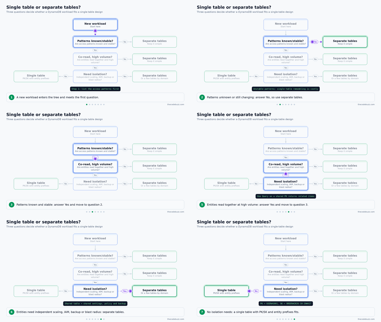
The table compares the two approaches across the main concerns.
| Concern | Single table | Separate tables |
|---|---|---|
| Scaling | Shared table settings | Tuned per entity |
| IAM and backup scope | One policy and one backup for everything | Separate policies, backups and blast radius |
| Change tolerance | New patterns may need remodeling or backfills | Easier to adapt |
| Readability | Harder; needs documented key conventions | Familiar, one entity per table |
How Do Vector Search and Large Blobs Affect Modeling?
Native vector search became generally available on Aug 5, 2026. Embeddings sit next to your other attributes, and a vector index type works alongside GSIs and LSIs. For many RAG and semantic-search cases, this removes the need for a second database. AWS claims single-digit millisecond latency at 99%+ recall, so verify that against your own data.
Keep large blobs (images, PDFs, long documents) in S3 and store only the reference in the item. Item size drives read and write units, so a lean item is cheaper to read and write. The cost section explains the arithmetic.
Partition Key, Sort Key and GSI Design: Avoid Hot Partitions
Choose a high-cardinality partition key (many distinct values) whose traffic spreads evenly, and use the sort key for ordering and range queries inside one item collection. AWS advises designing for uniform activity across all partition keys in the table and in its secondary indexes.
What are the per-partition limits in DynamoDB?
Each partition is designed to deliver up to 3,000 read units and 1,000 write units per second. Item size counts toward these limits.
- Read unit: one strongly consistent read per second, or two eventually consistent reads per second, for an item up to 4 KB.
- Write unit: one write per second for an item up to 1 KB.
Example: a 20 KB item costs 5 read units per strongly consistent read (20 / 4). About 600 reads per second on that single item uses 3,000 read units, which is the partition limit.
What does adaptive capacity fix, and what does it not?
Adaptive capacity works in both on-demand and provisioned modes and helps when traffic is uneven across keys. It cannot raise the hard per-partition limit for one hot key. Total throughput is still bounded by your provisioned throughput or the on-demand table limit.
In plain English: A hot partition is one checkout lane with a huge queue while the other lanes sit empty. Adding more lanes does not help if every customer insists on the same lane.
Which partition keys work and which fail?
The table below compares common choices for DynamoDB partition key design.
| Key | Why it works or fails | Fix |
|---|---|---|
| userId, orderId | Many distinct values, traffic spreads well. | Use as is. |
| date, timestamp | All current writes hit today’s key. | Move time to the sort key. |
| status, boolean | Only a few values, so a few partitions take everything. | Use a sparse GSI instead. |
| country | Low cardinality, skewed by population. | Combine with another attribute. |
| tenantId | Risky when one tenant is far larger than the rest. | Write-shard the large tenant. |
How do you design the sort key?
The sort key orders items inside one partition key and enables range queries. Use ISO 8601 timestamps or prefixed values such as ORDER#2026-10-25, because they sort correctly as strings. Sort keys compare as plain strings, so a longer value sorts after its shorter prefix.
- begins_with: fetch all items for one prefix, e.g.
ORDER#2026-10for a month. - between: fetch a date range. Both bounds are inclusive, so choose the upper bound with care (see the pitfall below).
- Composite sort keys: encode hierarchies such as
COUNTRY#IN#CITY#PUNEto query at any level.
Here is the pitfall. Suppose your sort keys look like ORDER#2026-10-25#A18 (date, then order ID). The condition BETWEEN 'ORDER#2026-10-01' AND 'ORDER#2026-10-25' silently drops every order placed on the 25th, because ORDER#2026-10-25#A18 is longer than the upper bound and sorts after it. The lower bound is safe, since a shorter prefix sorts before the longer keys that start with it.
There are two simple fixes. Use the next day as the upper bound (ORDER#2026-10-26), or add a high character such as ~ to the end of the day (ORDER#2026-10-25~). The ~ character sorts after #, digits and letters in byte order, so it works when order IDs are plain alphanumeric text.
Python
import boto3
from boto3.dynamodb.conditions import Key

table = boto3.resource("dynamodb").Table("Orders")

resp = table.query(
    KeyConditionExpression=Key("PK").eq("USER#u-1001")
    & Key("SK").between("ORDER#2026-10-01", "ORDER#2026-10-25~")
)
orders = resp["Items"]
This returns all orders from 1 October to 25 October 2026 for one customer, including those placed on the 25th.
How does write sharding spread a hot key?
Write sharding appends a calculated or random suffix (e.g. a hash of orderId modulo N) to one logical key. The trade-off is that reads become scatter-gather: you query all N shards and merge. The animated diagram below shows the write fan-out and the read path.
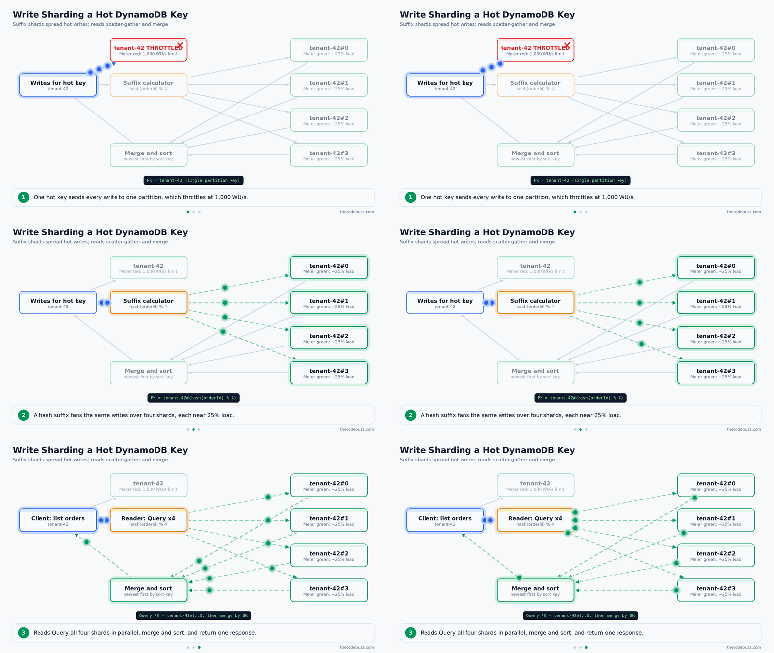
The simplified example below writes with a stable hash suffix and reads the newest orders from four shards. Python’s built-in hash() changes between processes, so use hashlib.
Python
import hashlib
import boto3
from boto3.dynamodb.conditions import Key

SHARDS = 4
table = boto3.resource("dynamodb").Table("Orders")

def shard_for(order_id: str) -> int:
    return int(hashlib.md5(order_id.encode()).hexdigest(), 16) % SHARDS

def put_order(tenant, order_id, created_at, attrs):
    table.put_item(Item={
        "PK": f"TENANT#{tenant}#{shard_for(order_id)}",
        "SK": f"ORDER#{created_at}#{order_id}",
        **attrs,
    })

def list_orders(tenant, limit=50):
    """Return the newest `limit` orders across all shards (first page only)."""
    items = []
    for shard in range(SHARDS):
        kwargs = {
            "KeyConditionExpression": Key("PK").eq(f"TENANT#{tenant}#{shard}"),
            "ScanIndexForward": False,
            "Limit": limit,
        }
        shard_items = []
        while len(shard_items) < limit:
            resp = table.query(**kwargs)
            shard_items.extend(resp["Items"])
            if "LastEvaluatedKey" not in resp:
                break
            kwargs["ExclusiveStartKey"] = resp["LastEvaluatedKey"]
            kwargs["Limit"] = limit - len(shard_items)
        items.extend(shard_items)
    items.sort(key=lambda i: i["SK"], reverse=True)
    return items[:limit]
Each shard is read only until it has limit items, so the function reads at most SHARDS × limit items. That is enough, because the newest limit orders overall must be among the newest limit of some shard. The LastEvaluatedKey loop is still needed because one query response is capped at 1 MB of data.
For a “next page” feature, keep one LastEvaluatedKey per shard and resume each shard from its own cursor. To fetch every order for a tenant instead, remove the limit check and expect to read all items on all shards. In production, run the shard queries in parallel.
What are the GSI best practices?
Add a global secondary index (GSI) only for a proven access pattern. Each GSI repeats every matching write, so it adds write cost and storage. Apply the same uniform-key rule to GSI keys, because a skewed GSI key can throttle writes to the base table.
- Sparse GSIs: only items that carry the GSI key attributes are copied. If only open orders have the key, the index stays small and cheap.
- Index overloading: use generic
GSI1PKandGSI1SKso one index serves several entity types. - GSI write sharding: shard the index key the same way as the table key.
- Narrow projections: use
KEYS_ONLYorINCLUDEinstead ofALLunless every attribute is needed.
How many GSIs should a table have? As few as your proven access patterns need. The default quota has been 20 GSIs per table, but quotas can change and can be raised on request, so confirm the current number on the DynamoDB quotas page for your Region and account.
What should you know about LSIs and the 10 GB item-collection limit?
A local secondary index (LSI) uses the same partition key as the base table with a different sort key. It must be defined when the table is created, and the default quota has been 5 LSIs per table (confirm on the quotas page).
If a table has an LSI, the 10 GB limit applies to each item collection, meaning all items (and their LSI entries) that share one partition key value. Writes to a collection that reaches the limit are rejected. Tables without an LSI don’t have this cap.
This is why an unbounded collection, such as every order for one tenant under a single partition key, is risky on a table with an LSI. Prefer a GSI when you need an alternate sort order, or bound collections with a time bucket or a shard suffix.
How do you keep queries cheap?
- Use Query, not Scan: Query reads one item collection, while Scan reads the whole table.
- Add ProjectionExpression: return only the attributes you need.
- Use eventually consistent reads: they cost half as much when slightly stale data is acceptable.
- Don’t treat FilterExpression as an index: it filters after reading, so you still pay for all the data read.
Transactions, Consistency, Replication and Streams
Use conditional writes for optimistic concurrency, use TransactWriteItems only where several items must succeed or fail together, and choose the replication model by the consistency you need.
How do conditional writes prevent overwrites?
Add a ConditionExpression to a write, and DynamoDB applies it only if the condition is true. Use attribute_not_exists(PK) to block overwriting an existing item. For optimistic locking, keep a version attribute and write with version = :expected, then increment it.
In plain English: A conditional write is like a ticket office checking the seat is still free at the moment you pay. If someone else took it first, your purchase is refused instead of silently replacing theirs.
When should you use TransactWriteItems?
TransactWriteItems is all-or-nothing across items. Keep it for cases such as moving an order status and writing a ledger item in finance. A transactional read costs 2 RRUs on-demand, against 1 for a strongly consistent read and 0.5 for an eventually consistent one.
C# (.NET)
using Amazon.DynamoDBv2;
using Amazon.DynamoDBv2.Model;

// Create one client per process and reuse it.
var client = new AmazonDynamoDBClient();

var orderId = Guid.NewGuid().ToString();

var request = new TransactWriteItemsRequest
{
    ClientRequestToken = orderId, // same token on retry = same request
    TransactItems = new List<TransactWriteItem>
    {
        new TransactWriteItem
        {
            Put = new Put
            {
                TableName = "AppTable",
                Item = new Dictionary<string, AttributeValue>
                {
                    ["PK"] = new AttributeValue { S = "USER#42" },
                    ["SK"] = new AttributeValue { S = $"ORDER#{orderId}" },
                    ["entityType"] = new AttributeValue { S = "Order" }
                },
                ConditionExpression = "attribute_not_exists(PK)"
            }
        },
        new TransactWriteItem
        {
            Update = new Update
            {
                TableName = "AppTable",
                Key = new Dictionary<string, AttributeValue>
                {
                    ["PK"] = new AttributeValue { S = "USER#42" },
                    ["SK"] = new AttributeValue { S = "PROFILE" }
                },
                UpdateExpression = "ADD orderCount :one",
                ConditionExpression = "attribute_exists(PK)",
                ExpressionAttributeValues = new Dictionary<string, AttributeValue>
                {
                    [":one"] = new AttributeValue { N = "1" }
                }
            }
        }
    }
};

try
{
    await client.TransactWriteItemsAsync(request);
}
catch (TransactionCanceledException ex)
{
    foreach (var reason in ex.CancellationReasons)
        Console.WriteLine($"{reason.Code}: {reason.Message}");
}
The order item and the customer counter commit together, or neither does. CancellationReasons tells you which condition failed.
How should you handle retries and pagination?
- Trust SDK retries: The SDKs retry throttled requests with backoff by default, so do not add custom tight retry loops.
- Reuse the client: Keep one client instance per process.
- Paginate: Loop on
LastEvaluatedKeyfor every Query and Scan.
Which replication model fits your consistency needs?
Global tables replicate across Regions. Multi-account global tables (announced Feb 3, 2026) add account-level isolation and separate governance. Multi-Region strong consistency (MRSC) is available in 15 AWS Regions as of the Sept 2026 expansion, so check your Regions first. In Oct 2026 AWS added replica disassociation, which lets a Region or account keep its table as a standalone single-Region table without copying data.
| Model | Read freshness | Write latency | Use case |
|---|---|---|---|
| Global table (eventual) | Remote Regions may lag briefly | Local, lowest of the multi-Region options | Active-active apps, local reads |
| Global table (MRSC) | Strongly consistent across Regions | Higher, because Regions coordinate | Finance, no stale reads after failover |
| Single Region | Strong reads within the Region | Lowest | Simple apps, one-Region compliance |
What changed in DynamoDB Streams?
Streams now supports the AT_TIMESTAMP shard iterator (announced Oct 15, 2026). A consumer can start from a point in time instead of only the oldest retained record (up to 24 hours old) or new records. It also works with KCL through the Streams Kinesis adapter.
In a single-table design, route stream consumers by the entityType attribute, so an order handler ignores customer records.
DynamoDB Cost Optimization: On-Demand vs Provisioned and Item Size
Start with on-demand for most workloads. Move to provisioned with auto scaling only when traffic is steady and predictable. Cut cost first by shrinking items and removing unused indexes, because those savings apply in every capacity mode.
Is on-demand or provisioned cheaper in DynamoDB?
After the November 2024 on-demand price reduction, on-demand is commonly the default recommendation. Before that price cut, on-demand was widely seen as much more expensive for steady workloads. Provisioned capacity with auto scaling can still save money for steady traffic, but the gap has narrowed.
In plain English: On-demand is like paying per taxi ride, so you pay only when you travel. Provisioned is like leasing a car: cheaper per trip if you drive every day, wasted money if it sits in the garage.
A secondary summary of the AWS cost-optimization page puts the break-even at about 35% average utilization of provisioned capacity. That figure has not been confirmed against the AWS documentation, so treat it as unverified. It also says on-demand can still win above that level when traffic has quiet periods with occasional peaks. Check the current AWS cost-optimization page and your own CloudWatch usage data before you decide.
The animated diagram below shows the decision path for choosing a capacity mode.

How do the capacity modes compare?
This table compares the three options across the main decision factors.
| Factor | On-demand | Provisioned | Provisioned + auto scaling |
|---|---|---|---|
| Traffic shape | New, spiky or unknown | Flat and known | Steady with gradual changes |
| Throttling risk | Low | High if under-provisioned | Medium; scaling reacts to load |
| Planning effort | None | High | Medium (targets and limits) |
| Cost behaviour | Pay per request | Pay for reserved units, used or not | Follows load, with some headroom |
AWS Database Savings Plans (launched December 2025) are a discount layer on top of a capacity mode, not a third mode. A 1-year commitment gives up to about 18% on on-demand throughput and up to about 12% on provisioned capacity.
What does a read cost on-demand?
Read cost depends on consistency and item size, in 4 KB steps. The table shows the on-demand read units (RRUs) per read of up to 4 KB.
| Read type | Cost (up to 4 KB) |
|---|---|
| Strongly consistent | 1 RRU |
| Eventually consistent | 0.5 RRU |
| Transactional | 2 RRUs |
For storage, the source quotes list prices of $0.25 per GB-month for Standard and $0.10 per GB-month for Standard-IA. Confirm prices for your Region on the AWS pricing page.
How do I compare the modes with my own numbers?
Convert your traffic into monthly units, then multiply by the list price for your Region. The formula is requests per second x units per request x seconds in the month x price per unit. This guide does not quote throughput prices, so take them from the AWS pricing page.
The example below uses a simplified workload: a retail catalog service that reads a 6 KB item with strongly consistent reads, averaging 100 reads per second with a peak of 200 reads per second. It assumes a 30-day month (2,592,000 seconds, 720 hours) and provisioned capacity set flat at the peak.
| Step | On-demand | Provisioned (flat at peak) |
|---|---|---|
| Units per read | 6 KB rounds up to two 4 KB blocks = 2 RRUs | 2 read units |
| Rate used | Average: 100 x 2 = 200 RRUs per second | Peak: 200 x 2 = 400 read capacity units |
| Monthly quantity | 200 x 2,592,000 = 518.4 million RRUs | 400 x 720 = 288,000 capacity-unit hours |
| Monthly cost | 518.4 x on-demand price per million RRUs | 288,000 x provisioned price per capacity-unit hour |
| Average utilization | Not applicable (pay per request) | 200 / 400 = 50% |
Plug both prices into the last row and compare the two totals. Repeat the same steps for writes, using 1 write unit per 1 KB. If you switch to eventually consistent reads, halve the read units in both columns.
This simplified Python script does the same arithmetic. It asks for the two prices so you can enter the current values for your Region, and you can add your own logic for writes or auto scaling.
Python
import math

SECONDS_PER_MONTH = 30 * 24 * 3600
HOURS_PER_MONTH = 30 * 24


def read_units(item_kb, strongly_consistent=True):
    """Read units for one read: 4 KB blocks, halved for eventual consistency."""
    blocks = math.ceil(item_kb / 4)
    return blocks * (1 if strongly_consistent else 0.5)


def compare_read_cost(avg_rps, peak_rps, item_kb, od_price_per_million, prov_price_per_unit_hour):
    units = read_units(item_kb)
    on_demand_units = avg_rps * units * SECONDS_PER_MONTH
    provisioned_unit_hours = peak_rps * units * HOURS_PER_MONTH
    return {
        "on_demand_cost": on_demand_units / 1_000_000 * od_price_per_million,
        "provisioned_cost": provisioned_unit_hours * prov_price_per_unit_hour,
        "avg_utilization": avg_rps / peak_rps,
    }


od_price = float(input("On-demand price per million read units: "))
prov_price = float(input("Provisioned price per read capacity unit-hour: "))
print(compare_read_cost(100, 200, 6, od_price, prov_price))
The script returns both monthly costs and the average utilization, so you can see which mode is cheaper for your traffic shape.
How do item size and GSIs multiply cost?
A write unit covers 1 KB, so a 6 KB item write costs 6 write units. A strongly consistent read of the same item costs 2 read units (6 KB rounds up to two 4 KB blocks). Every GSI that contains the item repeats the write.
The table shows write units for one 6 KB item under different designs. KEYS_ONLY figures assume the projected keys fit in 1 KB.
| Design | Write units per 6 KB item |
|---|---|
| No GSI | 6 |
| 3 GSIs, ALL projection, item in every index | Up to 24 (6 x 4) |
| 3 GSIs, ALL projection, item in only one (sparse) | 12 |
| 3 GSIs, KEYS_ONLY projection | About 9 (6 + 3 x 1) |
Which other levers reduce the DynamoDB bill?
- Standard-IA table class: Use it for data that is stored a lot but read rarely (e.g. old retail orders).
- TTL: Expire old items such as sessions so you stop paying to store them.
- Blobs in S3: Keep only a reference in the item to shrink read and write units.
- Short attribute names: Apply only where item size is truly the cost driver, since they hurt readability.
- Eventually consistent reads: Use them where slightly stale data is acceptable, to halve read cost.
- PITR and backups: Track their storage as its own line item on the bill.
DynamoDB Security, Backups, Monitoring, Anti-Patterns and Production Checklist
Turn on point-in-time recovery (PITR) and deletion protection, give each application least-privilege IAM access, and alarm on throttles before users notice them. DynamoDB has no servers to patch, so most of your production work is access control, recovery and watching the right metrics.
How do you secure a DynamoDB table?
Grant only the actions and keys each application needs, and keep traffic private. The points below cover the main controls:
- Least-privilege IAM: Scope policies to one table, and to specific actions such as
dynamodb:GetItemanddynamodb:Query. Avoiddynamodb:*on all tables. - Key-prefix access: Use the
dynamodb:LeadingKeyscondition key to limit a caller to partition keys it owns (e.g. one tenant’sTENANT#prefix in a SaaS product). - Encryption at rest: It is on by default. You do not need to enable it, but check which key type your compliance rules require.
- Private access: Use a VPC gateway endpoint so traffic from your VPC does not travel over the public internet.
- Account isolation: Keep production in its own account. Multi-account global tables help when replicas need separate governance.
- Sensitive data: Do not store secrets or unencrypted personal data (e.g. patient identifiers in a healthcare app) in plain attributes. Keep secrets in a secrets manager.
How do you back up and restore DynamoDB?
Use PITR for continuous recovery inside its retention window, and on-demand backups for long-term copies. Both add storage cost, so treat them as a budget line item.
Note : PITR is like a security camera that records continuously. If someone deletes the wrong rows at 2:10 PM, you rewind to 2:09 PM. It only keeps footage for a limited time, so older copies need on-demand backups.
The retention window is configurable. You set the recovery period in the same PITR specification (the RecoveryPeriodInDays field), so pick a window that matches how long it could take you to notice a bad deployment or a bad delete. Check the current AWS documentation for the allowed range, and remember that a longer window means more backup storage.
The commands below enable PITR and deletion protection on a table named Orders:
AWS CLI
aws dynamodb update-continuous-backups \
  --table-name Orders \
  --point-in-time-recovery-specification PointInTimeRecoveryEnabled=true

aws dynamodb update-table \
  --table-name Orders \
  --deletion-protection-enabled
The first command turns on continuous backups with the default retention window. The second blocks the table from being deleted until you switch protection off.
What does a DynamoDB restore bring back, and what do you reapply?
A restore always creates a new table. By default it brings back the data and the table’s GSIs and LSIs, but not auto scaling, IAM, alarms or TTL, so you must set those up again on the new table.
| Item | Restored? | What you do |
|---|---|---|
| Table data | Yes | Verify with spot-check queries |
| GSIs and LSIs | Yes, by default | Confirm they are present and active before sending traffic |
| Auto scaling settings | No | Reapply the scaling policies if you use provisioned mode |
| IAM policies | No | Update policies to the new table name and ARN |
| CloudWatch alarms | No | Recreate the throttle and error alarms |
| TTL setting | No | Enable TTL again on the expiry attribute |
Keep these settings in infrastructure-as-code so reapplying them is a repeatable step, not a manual checklist. Also check the AWS restore documentation for other table settings (e.g. stream settings and tags) that you may need to review. Rehearse the restore on a schedule so the first time you do it is not during an incident.
What changes for operations and upgrades?
Nothing needs patching. There are no OS settings, memory tuning, maintenance windows or version upgrades, because features ship continuously. Instead, review new announcements during architecture reviews (e.g. Streams AT_TIMESTAMP, vector search, replica disassociation).
Use TTL to expire old items. Expiry is not instant, so filter expired items in reads if stale data would cause problems.
Which metrics should you monitor?
Alarm on throttling and errors first, then watch consumption. Track ThrottledRequests, ReadThrottleEvents, WriteThrottleEvents, SystemErrors, ConsumedReadCapacityUnits, ConsumedWriteCapacityUnits and, for global tables, ReplicationLatency.
Enable CloudWatch Contributor Insights to see the most accessed and most throttled keys. It is the fastest way to confirm a DynamoDB hot partition.
What are the common DynamoDB anti-patterns?
This table maps each mistake to what you will see and how to fix it:
| Anti-pattern | Symptom | Fix |
|---|---|---|
| Timestamp or status as partition key | Throttling on a few keys | Use a high-cardinality key such as orderId |
| Scan in the request path | Slow reads, high read cost | Use Query with a purpose-built key or GSI |
| One GSI per idea | High write cost and storage | Keep only proven indexes; use sparse and overloaded GSIs |
| Blobs stored inline | Large items, expensive reads and writes | Store in S3, keep a reference |
| Unbounded item collection with huge items | One key grows and gets hot | Split the key or shard it |
| FilterExpression as an index | Paying to read data you discard | Model the filter into the key or a GSI |
| Single table on a simple, changing domain | Hard-to-read model, painful changes | Use separate tables |
| Over-provisioned capacity left unchanged | Low utilization, high bill | Review the capacity mode and auto scaling |
| No PITR or deletion protection | Accidental loss is permanent | Enable both |
| Hot tenant, no sharding | One large tenant is throttled | Add a write-shard suffix to the key |
Production readiness checklist
Work through these steps in order before go-live:
- List access patterns: Test each one with a real Query.
- Check key cardinality: Confirm traffic spreads evenly across partition keys.
- Justify every GSI: Document each index and its projection.
- Set an item size and blob policy: Decide what goes to S3.
- Choose the capacity mode: Document why.
- Enable PITR and deletion protection: Set the PITR retention window deliberately, and add TTL where data expires.
- Apply least-privilege IAM: Use
dynamodb:LeadingKeyswhere callers share a table. - Configure alarms: Alert on throttles, and enable Contributor Insights.
- Run a restore test: Check that the data and GSIs/LSIs are present, then reapply auto scaling, IAM, TTL and alarms from your infrastructure-as-code.
- Load-test the hottest key: Compare results with the per-partition limits.
Key takeaways
These are the points to remember from the guide, in the order you will usually need them.
- Design from access patterns first: list every read and write before you choose keys. Single-table design is a tool for known, related, high-volume patterns, not a universal rule. Use separate tables when entities scale or fail independently, or when patterns are simple or still changing.
- Use a high-cardinality partition key: one partition is designed for up to 3,000 read units and 1,000 write units per second, and item size counts toward that. Adaptive capacity helps with uneven traffic, but it cannot lift the cap for one hot key. Avoid timestamps and status values as partition keys, and use write sharding when one logical key is genuinely hot.
- Keep GSIs few, sparse and narrowly projected: every GSI repeats the write, so it adds write cost and storage. Add one only for a proven access pattern, and prefer KEYS_ONLY or INCLUDE over ALL. Apply the same even-spread rule to GSI keys, because a skewed index key can throttle base-table writes.
- Prefer Query over Scan: use
ProjectionExpressionand eventually consistent reads where staleness is acceptable.FilterExpressionis not an index, because you still pay for everything it reads before filtering. - Use the right tool for consistency: use conditional writes for optimistic concurrency, and
TransactWriteItemsonly when several items must succeed or fail together. Transactional reads cost more than normal reads. Pick the global table model (eventual consistency, MRSC or single Region) by the freshness you actually need. - Start on-demand, then measure: move to provisioned with auto scaling only when traffic is steady and predictable. Check the roughly 35% utilization break-even against the current AWS cost-optimization page and your own usage data, since it comes from a secondary summary. Database Savings Plans are a discount layer on top of a capacity mode, not a third mode.
- Treat item size as a cost driver: keep large blobs in S3 and store only the reference in the item. Use TTL to expire old data and Standard-IA for rarely read tables, and watch PITR and backup storage as a line item.
- Protect and observe the table: enable PITR and deletion protection, apply least-privilege IAM, and alarm on throttle metrics. Use Contributor Insights to confirm hot keys, and run restore tests on a schedule.
- Review new features when you revisit the design: DynamoDB has no versions, so check announcements such as multi-account global tables, MRSC, replica disassociation, Streams AT_TIMESTAMP and vector search. Each may simplify an architecture you built around older limits.
FAQ
Is single-table design always the best approach in DynamoDB?
No. Single-table design pays off when your access patterns are known, related and high volume, because one Query can return several entity types from the same partition key. Use separate tables when entities scale or fail independently, need separate IAM, backup scope or blast radius, or when the access patterns are simple or still changing.
How do I choose a good partition key in DynamoDB?
Choose an attribute with high cardinality (many distinct values) whose traffic is spread evenly, and that matches your main lookup, such as customerId or orderId. Avoid timestamps and status or boolean values, because they send most traffic to a few key values. Apply the same rule to the keys of your GSIs, since a skewed index key can throttle base-table writes.
What is a hot partition and how do I fix it?
A hot partition is a partition that receives more traffic than its limit, so requests get throttled even when the table as a whole is well under its capacity. Confirm it with CloudWatch Contributor Insights, which shows the most accessed and most throttled keys. Then fix it with a better partition key, write sharding (a calculated suffix that spreads one logical key across N keys), or caching for read-heavy keys. Adaptive capacity helps uneven traffic, but it cannot lift the hard limit for a single hot key.
What are the throughput limits per partition in DynamoDB?
A partition is designed to deliver up to 3,000 read units and 1,000 write units per second, and item size counts toward both limits. A read unit is one strongly consistent read (or two eventually consistent reads) per second for an item up to 4 KB. For example, a 20 KB item costs 5 read units per strongly consistent read, so about 600 reads per second on that one item reaches the partition limit.
Should I use on-demand or provisioned capacity?
Start with on-demand for most workloads, because it needs no capacity planning and has lower throttling risk for spiky traffic. Move to provisioned with auto scaling when traffic is steady and predictable. One secondary summary of AWS guidance puts the break-even at roughly 35% average utilization of provisioned capacity, so check that figure against the current AWS cost-optimization page and your own usage data. AWS Database Savings Plans are a discount on top of either mode, not a third mode.
That’s all! Happy coding! Did this DynamoDB best practices guide help you solve your design or cost issue? Please share your questions or experience in the comments below. Bookmark this page and share it with your team, and subscribe to TheCodeBuzz for more database best-practice guides.
Sources and further reading
- Best practices for designing and using partition keys effectively in DynamoDB (AWS Documentation (Amazon DynamoDB Developer Guide))
- Best practices – AWS Prescriptive Guidance (DynamoDB data modeling) (AWS Prescriptive Guidance)
- Amazon DynamoDB now supports real-time vector search (AWS What’s New)
- Amazon DynamoDB global tables now support disassociating replicas (AWS What’s New)
- Amazon DynamoDB Streams now supports timestamp-based stream processing (AWS What’s New)